STABILITY OF LC OSCILLATORS

For frequencies from 3 to 30 MHz

Olivier ERNST F5LVG

Back to the home page: many other documents on the radio are waiting for you

Update 2023   FRANCAIS

Books, like websites, usually contain a lot of information about amplifiers. Conversely, the subject of oscillators is approached superficially and the assemblies made are empirically designed from "kitchen recipes" (W. Hayward, W7ZOI, introduction to radio frequency design, ARRL). This lack of information concerning the oscillators is due to the theoretical difficulty of the subject which cannot be approached correctly by approximations of linear electronics.

For the radio amateur, this subject is however essential: the demodulation of a voice wave in single side band (SSB) or in telegraphy (CW) requires an oscillator. Any amateur radio station, even the simplest, therefore includes at least one oscillator whose frequency stability, over a short period, must not exceed 100 Hz, or better 50 Hz, the voice becoming unpleasant from this frequency shift in SSB. Commercial devices currently use DDS (Direct Digital Synthesis) after having used frequency synthesizers for many years. These techniques can be used to generate a stable frequency, but they are much more complex to make and require far more components than a simple oscillator based on an amplifier associated with a resonant circuit formed by a coil L and a capacitor C.

The art of the radio amateur is to achieve simple LC oscillators with sufficient frequency stability. The purpose of this article is therefore to expose the rules which make it possible to obtain a frequency-stable LC oscillator for frequencies below 30 MHz. These rules were established from reading multiple papers and 40 years of experience in building amateur receivers. Ten laws are scattered throughout this exposition. The first four describe the general laws on the stability of an oscillator. The following laws (5 to 10) describe the main points to follow to achieve a stable oscillator. Finally, a 25 MHz oscillator suitable for SSB reception will be described (frequency drift less than 30 Hz per hour).

Before getting to the heart of the matter, here are the 10 commandments that allow you to obtain a stable oscillator. If you follow them, the results will be there.

1 Tank circuit tuned by a large capacitance (> 1000pF).

2 For fixed capacitors, use only NPO capacitors. Above 10 MHz, do not use capacitors larger than 220 pF. Use several capacitors in parallel to obtain the desired value.

3 Quality coil: High Q, large wire diameter, mechanical rigidity, no exotic support, no ferrite core, length equal to half the diameter.

4 Use a stabilized power supply.

5 Avoid temperature changes as much as possible. Move hot components away from the oscillator.

6 Use silicon bipolar transistors (BJT) with a transition frequency above 5 GHz.

7 Use the Seiler oscillator with a high tuning capacitance (> 1000 pF) and a capacity divider formed by three capacitors of respective value 100 pF, 220 pF and 220 pF.

8 Do not load the resonant circuit, which requires the use of a separator stage at the output of the oscillator.

9 Do not demand significant power from the oscillator. If necessary, provide one or more amplifier stages following the separator stage.

10 Design a rigid mechanical construction.

1 STABILITY OF A PERFECT OSCILLATOR

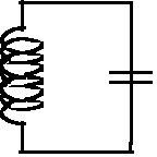
Figure 1: perfect resonant circuit

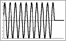
Figure 2: Voltage across a perfect resonant circuit as a function of time

Consider a perfect resonant circuit (CO) (figure 1). If the capacitor is charged by a voltage U, it discharges into the coil which then discharges into the capacitor etc... A sinusoidal voltage then exists at the terminals of the resonant circuit (figure 2). The frequency (fo) and the pulsation (ωo=2 π fo) of this sinusoid correspond to the equality of impedance between the capacitor and the coil. We therefore have Lωo = 1/Cωo, whence (ωo)² = 1/LC (Thomson's formula).

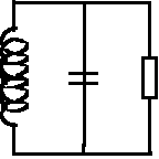
Figure 3: Real resonant circuit. Any connection of the resonant circuit in an assembly charges it, which is symbolized by the resistance in parallel.

Let us now study a perfect resonant circuit used in any assembly. This assembly will inevitably bring a resistance in parallel with the resonant circuit (figure 3). This resistance corresponds, for example, to the input resistance of an amplifier. This resistor will dampen the circuit and lower the resonant frequency. For example, in a perfect circuit (R = infinity), when the capacitor has discharged 10% of its energy, the coil is charged to 10% of the maximum energy. On the other hand, in the damped circuit, the capacitor will discharge into both the coil and the resistor. For the coil to have a charge equal to 10% of the maximum energy, it will therefore be necessary for the capacitor to have discharged more than 10% of its starting energy, for example 15% (10% of the energy charging the coil, and 5% of the energy being dissipated in R). As a result, the coil takes longer to reach 10% of the energy than in the ideal case without loss. In total, the oscillations are therefore slowed down and the resonance frequency decreases. The amplitude of the oscillations will also gradually decrease (Figure 4).

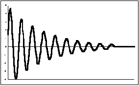
Figure 4: Evolution of the voltage at the terminals of a damped resonant circuit.

The damped frequency is lower than the undamped frequency

The lower the value of the load resistor, the lower the frequency of the oscillations. For an equal resistor value, the lower the capacitance, the greater the drop in frequency. For example, if C is halved (and L doubled), the capacitor will discharge twice as fast through the resistor. The result is the same as if the resistor value had been divided by 2. The decrease in pulse frequency of a loaded LC circuit (ωp) can be calculated mathematically: (ωp)² = (ωo)² – (1/2RC)². This formula confirms that the more a tank circuit is loaded (or damped) and the lower the value of the capacitance, the lower the pulsation frequency will be compared with the resonance frequency of a perfect oscillating circuit.

Now let's look at the oscillator circuit. The load resistor gradually decreasing the amplitude of the oscillations, it is essential to amplify them and then to reintroduce them on the resonant circuit to compensate for the losses. This is equivalent to introducing a negative resistance Rn in parallel with R. The frequency of the oscillations (fs,ωs) will then be greater than ωo. Let's go back to our example. When the capacitor has discharged 15% of its energy, the resistor has absorbed 5%. The coil is therefore charged to 10% of the starting energy to which must be added the energy reintroduced by the amplifier, for example 7%. The coil is then charged to 17% of the starting energy, whereas it would be charged to 15% for a perfect uncharged circuit and 10% for a damped circuit. In an oscillator, the energy transfers are therefore accelerated relative to an undamped resonant circuit, and the oscillation frequency is greater than ωo. In the formula giving ωp, it suffices to change the minus into plus to obtain ωs.

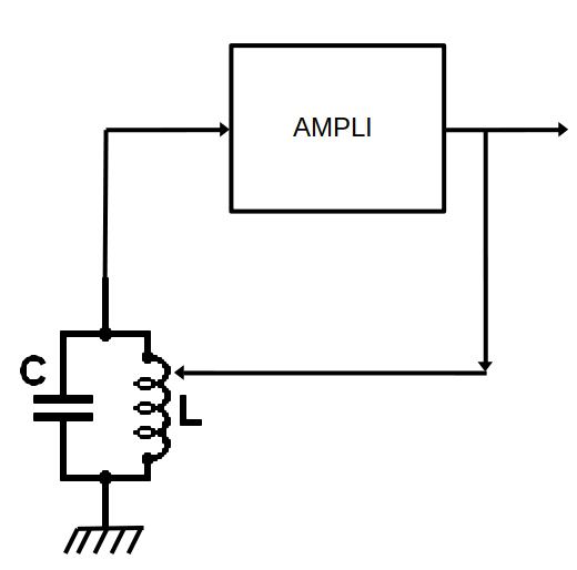
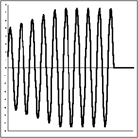
Figure 5: Theoretical diagram of an oscillator and evolution of the voltage at the terminals of the resonant circuit and at the output of the oscillator.

However, things are not so simple... Theoretically, the amplitude of the oscillations should increase indefinitely, which is materially impossible. After a certain time, the amplifier will be saturated: from a certain input voltage, the signal will be clipped, the resonance circuit charge will then be greatly increased, because the input resistance of the amplifier decreases sharply, most often by diode effect. After a certain time (theoretically infinite...), the oscillations will reach a constant amplitude (Figure 5). We then find ourselves in the case of the perfect resonant circuit, the oscillation frequency having gradually passed from ωs to ωo. The value of Rn is then equal to R due to the decrease in R.

The phenomenon of saturation of the oscillators is a plague for the radio amateur. After starting an oscillator, its frequency decreases progressively passing from ωs to ωo.On a direct conversion receiver, USB transmissions become increasingly high-pitched, and LSB transmissions increasingly low-pitched. To reduce this mechanism fs must be as close as possible to fo. The circuit must therefore be the least damped possible (R large), and the tuning capacity as large as possible. It is also desirable that the amplifier returns the minimum energy necessary on the resonant circuit so as to just compensate for the losses. In theory, if this compensation were perfect, we would have ωs = ωo, and therefore no frequency drift. However, an amplifier is never perfect and its gain fluctuates quite a bit.

To summarize this first part, let's remember that after start-up, an oscillator gradually decreases in frequency (law 1). To reduce this drop in frequency, the circuit must be lightly damped (low load) (law 2), the tuning capacitance must be high (law 3), and the amplifier must operate as far as possible from saturation, i.e. it must be set to class A. It is also possible not to connect the amplifier to the entire resonant circuit (see the Clapp and the Seiler below), which reduces the effect of saturation and variation of amplifier parameters.

2 REAL OSCILLATOR

2.1 Dependence between stability, frequency and capacity.

In a real oscillator, the characteristics of the different components vary during operation. Let's imagine that these modifications result in an increase in parasitic capacitances of 1% on an oscillator tuned to 7 MHz by a capacitance of 100 pF. The Thomson formula is used to calculate the ratio between the starting frequency (f1) and the frequency (f2) after increasing the capacitances by 1pF: (f1/f2)² = C2/C1 therefore (7/f2)² = 101/ 100 hence f2 = 6.965 MHz, a drop of 35 kHz. If the same oscillator is tuned to 14 MHz, the tuning capacitance must be 200 pF to maintain the same frequency variation after modification of 1 pF: (14/f2)² = 201/200 hence f2 = 13.965 MHz is again a variation of the frequency of 35 kHz.

This simple example illustrates that to maintain constant stability, the tuning capacity of an oscillator must be proportional to its frequency (law 4).

In practice, it is relatively "easy" to produce LC oscillators sufficiently stable in frequency for SSB and CW on frequencies below 10 MHz. This remains possible between 10 and 20 MHz, but relatively difficult. Between 20 and 30 MHz, an acceptable stability remains possible, but is rarely achieved.

2.2 Of the choice of the components of the resonant circuit of an LC oscillator (capacitor, coil).

The stability of an oscillator is based on the use of a tuning capacitor of very high value associated with a coil with very low loss.

2.2.1 Value of the tank circuit capacitor

To obtain constant stability, the value of the tuning capacitance must be chosen according to its frequency. Long amateur radio experience shows that to obtain sufficient stability to be able to listen to a SSB station for 10 minutes without altering the tuning capacity (cr), it is necessary: ​​cr pF > 50 f MHz (5r law). For a transmitter, it is preferable to use a double capacitance (ce): ce pF > 100 f MHz (5th law). It is necessary to add to these values ​​20% of adjustable capacity to precisely adjust the range covered.

However, a difficulty arises. At equal frequency, the lower the value of a coil, the lower its Q (quality coefficient), which at a certain value leads to an absence of oscillation. There is therefore a minimum value of the coil to be used, and therefore a maximum value of the tuning capacity to be adopted so that the assembly oscillates. The value of the maximum capacitance (cmax) to be used with a well-established circuit is inversely proportional to the frequency: cmax pF = k/F MHz (law 6). K is a constant which depends on the assembly and the amplifier element. For a bipolar transistor with Ft > 5 GHz, K = 20000. For a frame-gate tube, with a slope greater than 12 mA/V, k = 10000.

Let us remember that in practice the greater the capacitance of the resonant circuit, the more the oscillator will be stable in frequency. With bipolar transistors, it is possible to make LC oscillators with a tuning capacity of more than 1000 pF on 20 MHz.

Above 10 MHz, NPO ceramic capacitors of more than 220 pF should not be used to minimize their heating in operation and reduce RF losses, which facilitates oscillations. It is therefore necessary to put several capacitors in parallel to obtain the necessary capacitance value.

We should also mention an advantage of using a high capacitance value: the reduction in the hand effect when approaching the components of the oscillator. Indeed, our hand represents one of the 2 armatures of a bad capacitor made with it and the components. The larger the tuning capacitor, the smaller the frequency change as the hand approaches.

2.2.2 Tuning coil (self)

The secret of stability is therefore based on the greatest possible tuning capacity. This imposes a very low inductance value. It is essential that the loss resistance of the coil is very low compared to the impedance of the self or the capacitor so that the assembly can oscillate. It is therefore necessary to use an inductance with very low loss.

In practice, large diameter wire is required. To fix ideas, as soon as there are at least 5 turns, I use PVC insulated wiring wire with an external diameter of the cable of 1.1 mm, the diameter of the conductor 0.5 mm, and its section 0.2mm². For 4 turns and less, I use 20 A (2.5 mm²) electrical wire. The limit of the 2 techniques is around 9 MHz. The turns are contiguous and I do not use any coil form. When the coil is finished, after testing, I glue it with super glue (cyanolite). The coil must be perfectly rigid.

The resonant circuit of an oscillator must be tuned by a strong capacitance. The frequency of the oscillation will therefore be significantly lower than the resonance frequency of the coil (resonance of the coil tuned by its parasitic capacitances alone). In this case, the best length to diameter ratio will be 0.5 (Frederick Terman, Radio Engineers Handbook, McGraw-Hill, 1943, p74). In practice, the length of the coil should not be greater than its diameter.

As an illustration, I was able to obtain the zero beat of an oscillator on 20.7 MHz with a standard receiver for 3 hours, after more than an hour of warm-up. It was a tube oscillator (6K8) whose resonant circuit consisted of 2 turns of 20 A wire (2.5 mm²) over a diameter of 15 mm and the fixed capacitor was a 470 pF NPO capacitor. The 5 turn trickle coil used the 0.2mm² wiring wire.

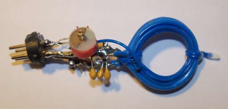
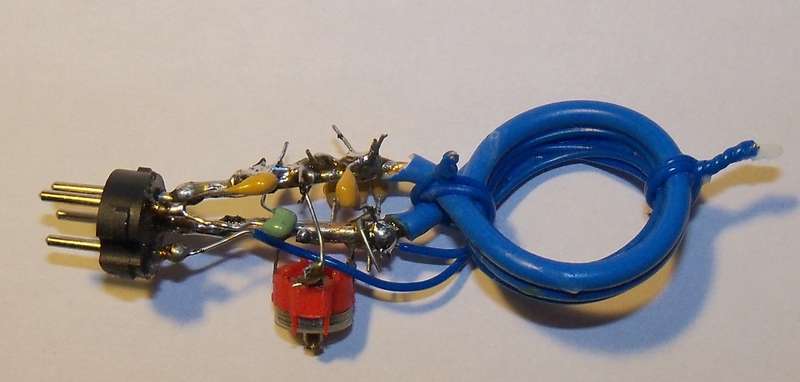
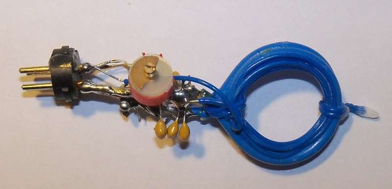
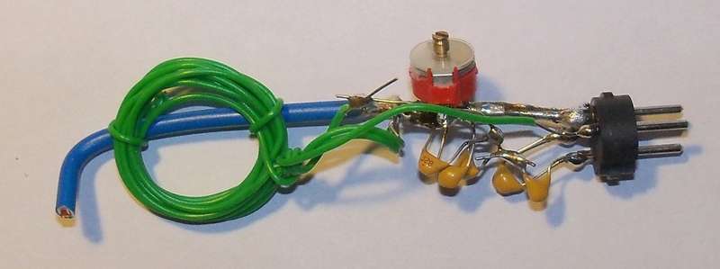
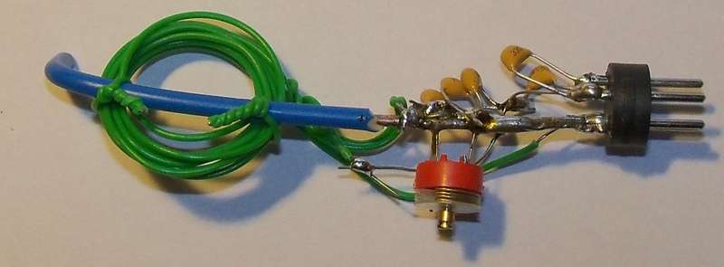
Making interchangeable plug-in coils is easily done using 4-pin DIN sockets. A few photos show the simplicity of this technique which makes it possible to obtain excellent quality chokes for frequencies from 3 to 30 MHz. You will notice that the entire resonant circuit is interchangeable: coil, fixed capacities, adjustable capacity. If a variable capacitor is required, it cannot be interchangeable.

2.3 Choice of transistor

To maintain good stability, the transistor must have a high input resistance. A double-gate MOSFET transistor is therefore highly desirable. Indeed, the impedance of a single-gate FET decreases sharply when the frequency increases. The input impedance of a BF245 at 10 MHz can thus be less than 3 kohm. It is also possible to employ a bipolar transistor having a transition frequency of at least 5 GHz. A non-decoupled 100 to 500 ohm feedback resistor in series with the emitter sometimes improves frequency stability due to an increase in input impedance (at the cost of lower slope). It is not useful with transistors having a transition frequency in the GHz.

In all cases, the transistor must operate in UHF (law 7) in order to present the lowest possible parasitic capacitances, and a high input impedance in HF. Personally, I sometimes use a double-gate UHF MOSFET (BF960), or more often a bipolar jonction transistor (BFR90, BFR91A or BFG541). The use of a transistor that does not operate in UHF, even if it is intended for VHF (example BF981) is nonsense... Due to the use of a UHF transistor, there is a risk of UHF oscillations added to HF oscillations. To avoid this phenomenon, it suffices to put a VHF choke coil or a resistor in series with the drain (collector) of the transistor. This type VK2OO choke can be replaced by a resistance of 100 ohms for FETs and 1 kOhm for bipolar transistors.

When using double-gate MOSFETs, it is essential not to forget to bias the transistor in such a way as to allow significant oscillation before the saturation phenomenon. Many assemblies carry out this polarization by putting a diode between gate 1 and ground. The polarization then takes place by rectifying the oscillation, which causes a load on the circuit, and therefore additional instability. This diode was recommended in the ARRL Hanbooks for more than 20 years, before being clearly discouraged in the 2000 edition, thanks to the work of Ulrich Rohde, KA2WEU. This recalls the need for radio amateurs to know, even today, how to get out of preconceived ideas, as our elders knew how to do. It is therefore preferable to carry out the polarization by a resistor in series with the source (law 8). This resistor will have the highest possible value that allows the system to oscillate (1 kohm for the BF960). Often it avoids the use of a choke coil in the source (emitter) circuit.

I often use bipolar transistors. I had the opportunity to study the frequency stability of an 18 MHz LC oscillator using either an SS9018 transistor or a BFR90 transistor. The stability obtained was significantly better with the  BFR90 than with the SS9018 , the drift being reduced approximately by 3. This illustrates the importance of employing a bipolar transistor with the highest possible transition frequency Ft and the collector capacitance as low as possible. In practice, it is necessary to use a silicon bipolar transistor with a transition frequency Ft greater than 5 GHz (BFR90, BFR91, BFG541, etc.).

2.4 Choice of other components

The fixed capacitors determining the frequency of an oscillator must be perfectly stable in temperature (NPO). Polystyrene capacitors (MKS, or styroflex) are expensive. NPO multilayer ceramic capacitors are small in size and relatively easy to find on the web. There are assortments of these capacitors allowing you to easily design your assemblies (Multilayer Ceramic Capacitors Assortment Kit NPO). Below 10 pF, many ceramic capacitors are NPOs.

Quality trimmer capacitors are extremely expensive today. I usually replace them with 2 or 3 capacitors fix NPO in parallel to get the desired value.

Variable capacitors are currently difficult to find, except to use small plastic capacitors intended for AM FM receivers. The 443DF model is still accessible (2X20 pF and 2X120 pF). They do not have a reduction drive. It is therefore necessary to provide a vernier. The frequency ranges must be subdivided into segments of approximately 150 kHz to achieve achievable tuning with the main capacitor and vernier.

The amateur ranges being small, it is possible to use varicaps. However, the voltage must be extremely well stabilized. High capacitance diodes (1SV149 for example) should be favored in HF, with a capacitor in series to limit the variation to the desired value. A 10-turn potentiometer provides sufficient spread. In VHF, to cover the 144, a simple BFR91a type UHF transistor mounted as a diode (emitter base or collector base) is satisfactory. In any case, the voltage must be perfectly regulated.

The coils can be made by any radio amateur who has a grid-dip or an LC meter (example model LC200A). It is not recommended to use a magnetic core.

2.5 What kind of oscillator circuit?

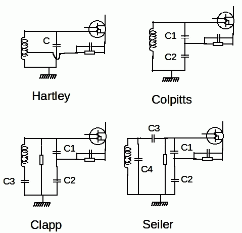
Figure 6: Different types of oscillators.

From a theoretical point of view, all oscillators are almost equal (figure 6). It is, however, not recommended choosing circuits with 2 transistors because of the imperfect phase shift provided by each transistor. The easiest to use with an OM build coil is the Hartley . The Colpitts is still a little easier due to the absence of a tap on the coil, the optimum location of this tap being critical for the Hartley. The resulting value of the two capacities of the Colpitts must, of course, have the value calculated by the theory, because of their serialization.

The Clapp is even better, but harder to tune. It is a Colpitts which is added in series between the coil and the ground a capacitor C3. There is therefore a capacitive divider between C3 and the resultant C1-C2. If for example C3 is 5 times weaker than the resultant C1-C2, the variations of capacities and the damping brought by the transistor (or the tube) will be 5 times weaker. We therefore have the equivalent of a standard Colpitts with a tuning capacity 5 times higher than the resultant C1-C2. The inductance of the coil should be 5 times higher than with the standard Colpitts.

The Seileris another variation of a capacitive divider. A simple example easily shows the interest of this assembly. Consider an LC oscillator tuned to 7 MHz with a capacitance of 100 pF. With a simple assembly like a Colpitts where the transistor is at the terminals of the entire resonant circuit, a variation of 1 pF brought by the transistor brings a variation of 35 kHz (see above). Consider a Seiler assembly with C1=C2=220pF, C3=50pF, and C4=65.625pF. The total resultant for the tuning capacitance therefore remains 100 pF. As before, the transistor brings a variation of 1 pF to the terminals of C1-C2. The resultant of C1-C2 becomes 111 pF instead of 110 pF. The resultant of C1-C2-C3 goes from 34.375 pF to 34.472 pF. The tuning capacitance becomes equal to 100.097 pF. The variation in the tuning capacitance value has gone from 1 pF to 0.1097 pF, ie ten times less. The frequency variation decreases in the same proportions: 35 kHz to 3.4 kHz. To have the same effect with a Colpitts assembly, the tuning capacitance should be 1000 pF. If capacitor C3 is 100 pF, the capacitance variation of 1 pF at the terminals of the transistor results in a capacitance variation of 0.225 pF at the terminals of the resonant circuit. Note that the variable capacitor is placed in parallel with C4. The Seiler is relatively easy to tune maintaining a large total tuning capacitance (approximately 1000 pF) and a moderate capacitive divider bridge (eg 100 pF, 220 pF and 220 pF).

The resistor value between gate 1 and ground is 220 kohms (non-critical). To cover an amateur band, I recommend a Seiler. Note that it is sometimes necessary to put a choke coil (L = 1mH) in series between the source resistor and ground for Colpitts, Clapp and Seiler. This coil avoids damping the resonant circuit by this resistance.

The circuit for coupling the oscillator to the next stage must also be perfectly designed in order to load the resonant circuit to a minimum. A common collector (drain) stage is usually required. The coupling to the resonant circuit is generally done on the intermediate tap of the coil or of the capacitors C1-C2.

2.6 Effect of heat

Temperature variations cause all materials to expand or shrink. The characteristics of the components, and in particular their capacity, change. A change in temperature therefore causes a change in the frequency of oscillation. No significant source of heat should therefore be in the oscillator box. Voltage regulators should be far enough away from the oscillator. It is preferable that the main power supplies are entirely independent of the assembly where the oscillator is used.

2.7 Effect of supply voltage

A variation in the supply voltage leads to a variation in the internal capacities of a transistor. The supply voltage of an oscillator must therefore always be regulated, at least by a zener diode. A varicap will require a second regulator in series (Law 9). Ready-made regulator integrated circuits are generally very suitable.

2.8 Effect of harmonics

The harmonics of a well-designed oscillator do not generally affect the stability of an oscillator. Only one exception exists. These are transmitters whose output frequency is a multiple of the oscillator frequency. This type of construction was common on AM and CW transmitters from the 1930s to the 1960s. In this case, the local oscillator receives feedback from the HF output which is a high power harmonic. The oscillator will then attempt to synchronize to its harmonic. Certainly, the ratio between the frequency of the oscillator and the output frequency is always constant, but the ratio between their phases varies due to the intermediate resonant circuits which are never perfectly tuned. The oscillator will therefore try to get in phase with its harmonic, by changing its frequency. The output frequency therefore varies and will again modify the frequency of the oscillator. This phenomenon results in frequency instability. The synchronization on the harmonic is done all the more when the HF return on the oscillator is important and therefore when the output power is important and the antenna feeder is not shielded (long wire antenna). To avoid such sources of instability, never design a transmitter whose output frequency is a harmonic of the oscillator (law 10). It is therefore necessary to build a VFO with frequency change.

2.9 Mechanical realization

The mechanical realization must be rigid. Flying leads should not exist. The turns of the coils must be well fixed with a little cyanolite glue. There should never be a switch on an oscillator circuit. If it is essential to change the range, it is preferable to make one oscillator per range and to switch their output and their power supply. Besides the benefit of avoiding the commutator problem, this allows the oscillator to be optimized for each range. A metal box to avoid the hand effect (frequency variation when the hand approaches) and HF returns is almost essential.

2.10 Bandwidth covered

This presentation shows that an optimum result is obtained for a precise frequency. It is therefore not desirable to want to cover wide ranges with an amateur realization. It is preferable to cover a small frequency range (10% of the average frequency), which unfortunately makes it possible to cover the amateur bands without difficulty.

2.11 Choice of link capacity

The theoretical explanations given in paragraph 1, assumed that the transfer of energy on the resonant circuit was perfectly in phase with the original signal present in the resonant circuit. Consider the diagram in Figure 7a. In most books, it is advised to choose the lowest possible CL coupling capacitance, so that the impedance changes of the transistor during operation are negligible compared to the CL impedance. It is true that a low value of CL makes the frequency variations due, for example, to changes in the supply voltage of the transistor negligible. On the other hand, the experiment shows that the lower the value of CL, the more the frequency drift as a function of time increases. We therefore obtain exactly the opposite of what was expected. This is easily explained. Let Ri be the internal resistance between base and emitter of the transistor. CL is in series with Ri. There is therefore a discrepancyα at the terminals of Ri such that α=-arctg(ZCL/Ri). If the impedance of the capacitor is equal to the value of Ri, the phase shift is 45°. If the value of the impedance of CL is equal to 0.1 Ri the phase shift is 5°. The phase shift reaches 1° for a value of Cl equal to 0.02 Ri. If the transistor of Figure 7a is a BFR91A, with a collector current of 1mA, the value of Ri is 1Kohm. At 10 MHz, the impedance of a 16 pF capacitor is 1Kohm. If CL is 16 pF, the voltage present on the base of the transistor is 45° out of phase with respect to the initial signal. The signal reinjected into the resonant circuit by the transmitter is therefore out of phase (late) by 45° with respect to the initial signal. Due to this delay, the frequency of the oscillator decreases. This phenomenon theoretically continues for an infinite time.

The solution is to use a high value for CL, in practice at least 470 pF (law 11). To reduce the load brought to the resonant circuit by the transistor, it suffices to put in series with the emitter a resistance RE of 220 ohms. In our example, Ri then rises to 10 Kohms. The resulting diagram is given in Figure 7b. Note that this value could only have been obtained with CL of 1.6 pF in the absence of RE. But the assembly would probably not oscillate because of the significant phase shift (84°).

The adaptation to a MOSFET is given in FIG. 7C. The simplest is to remove CL and use RE for the transistor impedance increase and for its biasing. Despite the high input impedance of a MOSFET, RE remains indispensable. Indeed, at saturation, its impedance decreases sharply, RE then makes it possible to maintain an acceptable value.

The examples given in this paragraph make it possible to obtain sufficient stability for SSB reception on 14 MHz, the tuning capacitance of the resonant circuit being composed of a varicap, an adjustable of 90 pF, and a fixed capacitance of 220pF.

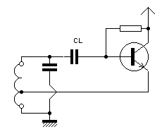
Figure 7a, what not to do: choose the minimum value for CL so that the transistor loads the resonant circuit as little as possible. Indeed, a low value of CL leads to a significant phase shift, the source of an almost infinite frequency shift.

Figure 7b, what to do: choose a large value for CL in order to make the phase shift that it introduces negligible. The charge brought by the transistor is reduced by RE. Note the presence of RL which is used to avoid self-oscillations in UHF, frequent with a UHF transistor. In practice CL = 470 pF, RE and RL = 220 Ohm.

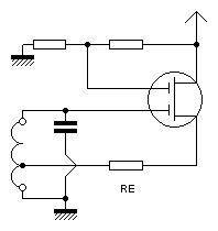
Figure 7c: Adaptation to a MOSFET. Notice that G1 is connected directly to the resonant circuit. The usual value of RE is 220 Ohm.

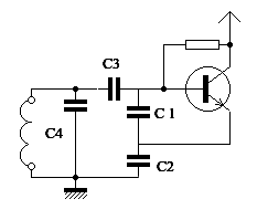
Figure 8: The Seiler assembly allows the transistor to be connected only to part of the resonant circuit due to the capacitive divider C3-C1-C2. The impedance variations of the transistor are therefore reduced on the resonant circuit. This assembly, which combines high tuning capacity and low coupling of the transistor to the resonant circuit, is recommended.

In the Clapp or Seiler assemblies (figure 8) C3 is part of the resonant circuit. The above considerations do not apply. The weaker C3 is, the less the transistor loads the resonant circuit, the more the oscillator is stable in frequency. There is, however, a minimum value, below which the transistor will not oscillate.

3 Example of a realization

I made a simple superheterodyne receiver for the amateur bands 80 40 20 17 and 15 m with an IF frequency of 4.5 MHz. It was therefore necessary to build a local oscillator covering from 8 MHz (3.5 MHz + 4.5 MHz) to 25.950 MHz (21.450 MHz + 4.5 MHz). It is a simple receiver, with interchangeable coils on DIN plugs.

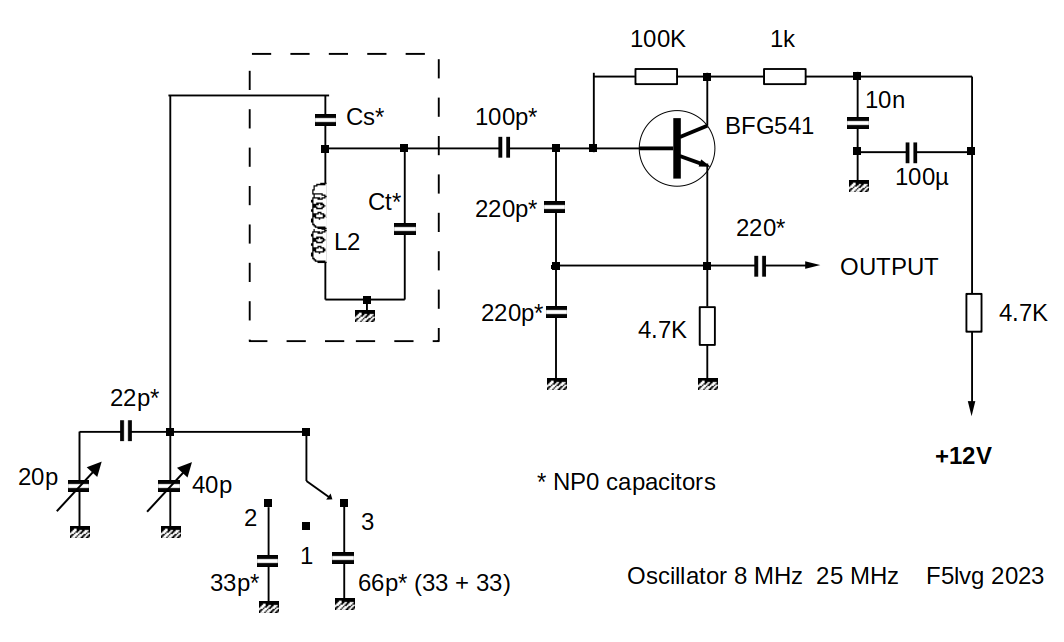
The circuit chosen is a Seiler. The bipolar transistor is a BFR90 or a BFG541. The 1kOhm resistor in the collector of the transistor serves to avoid UHF self-oscillations. For frequencies below 20 MHz, it is necessary to obtain a total tuning capacity of the resonant circuit greater than 1000 pF. The capacitors forming the capacitive divider for coupling to the transistor will be 100 pF, 220 pf and 220 pf. The 12V power supply is stabilized.

Two 443DF variable capacitors are used. These capacitors have no reduction drive. The main capacitor uses the 2 cages 20 pF (= 40 pF). The second capacitor serves as a fine tuner (vernier) using a single 20 pF cage in series with a fixed 22 pF capacitor. Finally, the amateur bands are subdivided into 3 sub-bands by a 3-position switch which brings 0 pF 33 pF or 66 pF in parallel with the 40 pF variable capacitor. By using large knobs (A05 knob) precise station tuning is possible on the vernier. 2.5 mm screws (2.5X25) are used to fix the buttons on the axis of the variable capacitors. Connections should be as short as possible.

Almost all of the resonant circuit is interchangeable on a DIN plug. Only the 3 capacitors of the capacitive divider and the capacitors used for tuning are not interchangeable. The coils are made with 20 A (2.5 mm²) installation wire. Refer to paragraph 2.2.2 for the practical realization of the coils. Capacitor Ct includes all the fixed tuning capacitance formed by several capacitors in parallel. The Cs capacitor is used to spread the amateur bands as much as possible. There is no adjustable capacitor. Several trials are necessary to obtain the result. The values ​​given in the table will probably be different due to a different construction. They give you an order of magnitude.

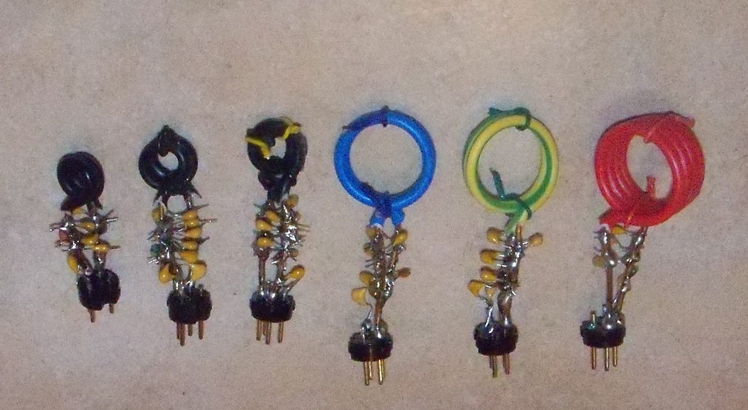
Photo of the resonant circuits interchangeable from the highest frequency to the lowest frequency.

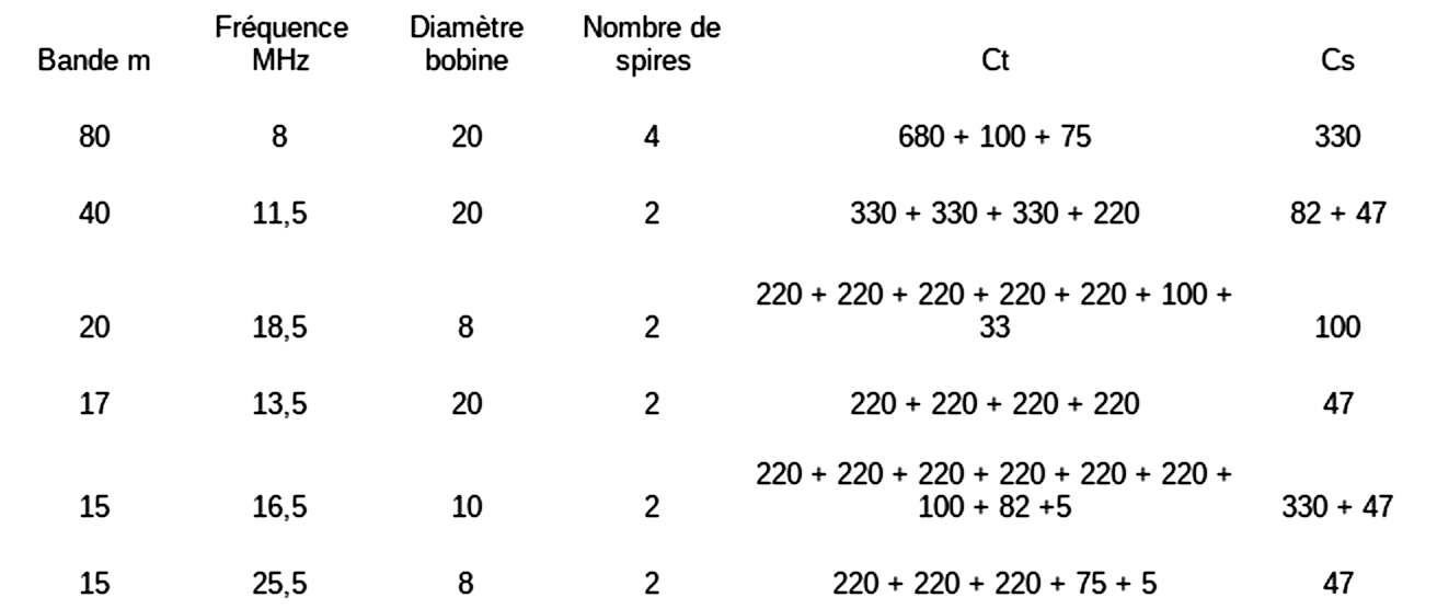
Depending on the bands, the oscillator is set below or above the frequency to be received (see the table) in order to keep the minimum value of 1000 pF for tuning. The 2 cases were carried out for the 21 MHz. Routinely, the 16.5 MHz resonant circuit is used. The 25.5 MHz circuit was made to test the oscillator above 20 MHz. Several tests have shown that the oscillator on the 25.7 MHz frequency remained at zero beat with a standard receiver for more than an hour (frequency drift not exceeding 30 Hz). There is no hand effect at 5 cm from the coil. It is therefore not necessary to provide shielding around the interchangeable resonant circuits. It is enough that the knobs are at more than 5 cm from the coil.

Olivier ERNST F5LVG

Back to the home page: many other documents on the radio are waiting for you